39 scatter chart in excel with labels
Find, label and highlight a certain data point in Excel ... To let your users know which exactly data point is highlighted in your scatter chart, you can add a label to it. Here's how: Click on the highlighted data point to select it. Click the Chart Elements button. Select the Data Labels box and choose where to position the label. Wrap category names (Y axis labels) of a scatter chart ... The labels are the standard axes labels and you have very limited control over their layout. You can add line feeds to wrap the text by adding ALT+ENTER to the text in the cells. If you want full control you will need to create your own textboxes to use as labelling. Register To Reply Bookmarks
Labelling of XY scatter charts in Excel 365 not downward ... See screenshots… first a snippet of how a simple test file looks in Excel 365, as it should; then a copy-paste image from the very same chart from the very same file: labelling is lost and replaced by "CELLRANGE"… (! yes indeed! even pasting the chart's image over doesn't work, and yes indeed, this is how it looks in Excel 2010).
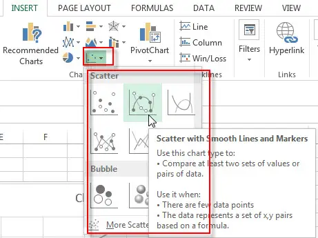
Scatter chart in excel with labels
How to Create a Quadrant Chart in Excel - Automate Excel We're almost done. It's time to add the data labels to the chart. Right-click any data marker (any dot) and click "Add Data Labels." Step #10: Replace the default data labels with custom ones. Link the dots on the chart to the corresponding marketing channel names. To do that, right-click on any label and select "Format Data Labels." How to display text labels in the X-axis of scatter chart ... Display text labels in X-axis of scatter chart Actually, there is no way that can display text labels in the X-axis of scatter chart in Excel, but we can create a line chart and make it look like a scatter chart. 1. Select the data you use, and click Insert > Insert Line & Area Chart > Line with Markers to select a line chart. See screenshot: 2. How to use a macro to add labels to data points in an xy ... In Microsoft Office Excel 2007, follow these steps: Click the Insert tab, click Scatter in the Charts group, and then select a type. On the Design tab, click Move Chart in the Location group, click New sheet , and then click OK. Press ALT+F11 to start the Visual Basic Editor. On the Insert menu, click Module.
Scatter chart in excel with labels. Labeling X-Y Scatter Plots (Microsoft Excel) When he creates an X-Y scatter chart (column B against column C) the result, as desired, is a graph showing an array of points showing the location of the objects. However, Martin can't seem to label the data points with their individual names (from column A). Present your data in a scatter chart or a line chart Select the data that you want to plot in the line chart. Click the Insert tab, and then click Insert Line or Area Chart. Click Line with Markers. Click the chart area of the chart to display the Design and Format tabs. Click the Design tab, and then click the chart style you want to use. Click the chart title and type the text you want. How to Make a Scatter Plot in Excel with Two Sets of Data? To get started with the Scatter Plot in Excel, follow the steps below: Open your Excel desktop application. Open the worksheet and click the Insert button to access the My Apps option. Click the My Apps button and click the See All button to view ChartExpo, among other add-ins. Scatter Plots in Excel with Data Labels Oct 29, 2020 · Select "Chart Design" from the ribbon then "Add Chart Element" Then "Data Labels". We then need to Select again and choose "More Data Label Options" i.e. the last option in the menu. This will...
Add Custom Labels to x-y Scatter plot in Excel ... Step 1: Select the Data, INSERT -> Recommended Charts -> Scatter chart (3 rd chart will be scatter chart) Let the plotted scatter chart be Step 2: Click the + symbol and add data labels by clicking it as shown below Step 3: Now we need to add the flavor names to the label.Now right click on the label and click format data labels. Under LABEL OPTIONS select Value From Cells as shown below. how to make a scatter plot in Excel — storytelling with data Highlight the two columns you want to include in your scatter plot. Then, go to the " Insert " tab of your Excel menu bar and click on the scatter plot icon in the " Recommended Charts " area of your ribbon. Select "Scatter" from the options in the "Recommended Charts" section of your ribbon. Change hover label data on Scatter plot chart | MrExcel ... Hi, I have 8 scattered plot charts, all containing more than 300 dots.. This means that I cant use ordinary labels, because it destroys all visibility of the chart. So I need to hover the dots to see the label data. This works good but I cant manage to get the names of the items on the hovering label. Excel scatter chart using text name - Access-Excel.Tips Since Excel allows different chart types to be displayed in one chart, we are going to create a mix of bar chart (column chart) and scatter chart. Scatter chart is used to display the actual data point, while bar chart is to display Grade labels. - Create scatter chart for Range B20:C31 (Series 1)
What is a 3D Scatter Plot Chart in Excel? - projectcubicle A 3D scatter plot chart is a two-dimensional chart in Excel that displays multiple series of data on the same chart. The data points are represented as individual dots and are plotted according to their x and y values. The x-axis represents time, while the y axis represents the value of the data point. When you create a 3D scatter plot chart ... Creating Scatter Plot with Marker Labels - Microsoft Community Right click any data point and click 'Add data labels and Excel will pick one of the columns you used to create the chart. Right click one of these data labels and click 'Format data labels' and in the context menu that pops up select 'Value from cells' and select the column of names and click OK. How to Add Labels to Scatterplot Points in Excel - Statology Sep 02, 2021 · Step 3: Add Labels to Points. Next, click anywhere on the chart until a green plus (+) sign appears in the top right corner. Then click Data Labels, then click More Options…. In the Format Data Labels window that appears on the right of the screen, uncheck the box next to Y Value and check the box next to Value From Cells. Improve your X Y Scatter Chart with custom data labels May 06, 2021 · Select the x y scatter chart. Press Alt+F8 to view a list of macros available. Select "AddDataLabels". Press with left mouse button on "Run" button. Select the custom data labels you want to assign to your chart. Make sure you select as many cells as there are data points in your chart. Press with left mouse button on OK button. Back to top
Excel scatter Chart - Free Excel Tutorial
How to Make a Scatter Plot in Excel | GoSkills A scatter plot (also known as an XY chart) is a type of chart that shows whether there is a relationship between two variables. It's one of the many chart types available in Excel . With this type of graph, one variable is plotted on the horizontal axis and the other on the vertical, and any resulting pattern is used to determine what kind of ...

Excel-Access.tips: Excel scatter chart using text name
Scatter chart horizontal axis labels | MrExcel Message Board If you must use a XY Chart, you will have to simulate the effect. Add a dummy series which will have all y values as zero. Then, add data labels for this new series with the desired labels. Locate the data labels below the data points, hide the default x axis labels, and format the dummy series to have no line and no marker. Click to expand...
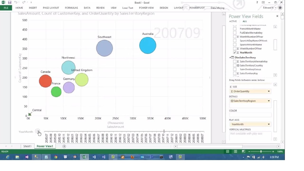
Excel 2013 PowerView Animated Scatterplot/Bubble Chart Business Intelligence Tutorial - YouTube
Use text as horizontal labels in Excel scatter plot ... Edit each data label individually, type a = character and click the cell that has the corresponding text. This process can be automated with the free XY Chart Labeler add-in. Excel 2013 and newer has the option to include "Value from cells" in the data label dialog. Format the data labels to your preferences and hide the original x axis labels.

Line Graph, Bar Graph, Scatter, Etc. | University of Denver
Scatter chart excel how to label the points - harewdelta In Microsoft Office Excel 2007, follow these steps:Ĭlick the Insert tab, click Scatter in the Charts group, and then select a type. In the Chart Wizard - Step 4 of 4 -Chart Location dialog box, click the As new sheet option, and then click Finish. In the Chart Wizard - Step 3 of 4 - Chart Options dialog box, click Next.
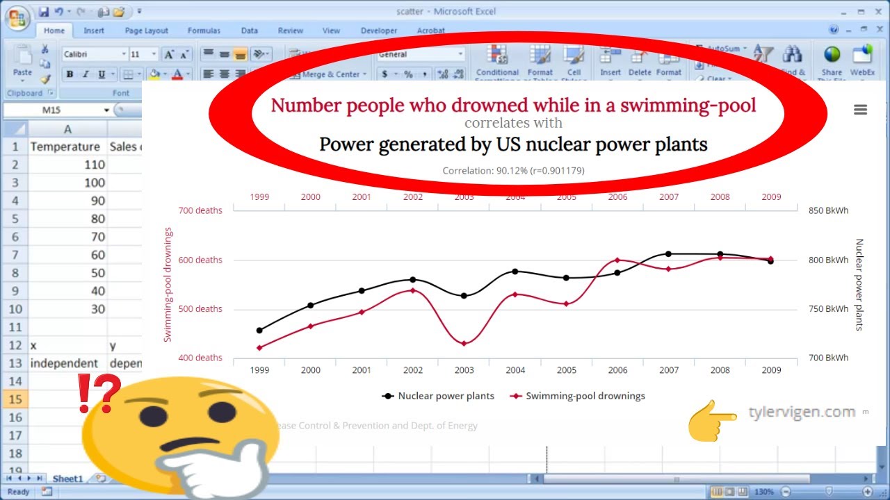
Create an X Y Scatter Chart - YouTube
Change the scale of the vertical (value) axis in a chart Because the scale of the line chart's horizontal (category) axis cannot be changed as much as the scale of the vertical (value) axis that is used in the xy (scatter) chart, consider using an xy (scatter) chart instead of a line chart if you have to change the scaling of that axis, or display it as a logarithmic scale.
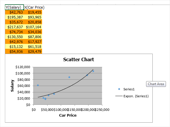
Create Excel Scatter Chart in C#
r/excel - Scatter Plot with Text Labels on X-axis You can replace chart labels with a different range of values, pretty neat. 1 level 1 · 5 yr. ago 1793 Excel doesn't support text labels for x-axis on scatter plots natively, so you have to fake it like so. Basic procedure is here. 1 level 1 · 5 yr. ago Hi! You have not responded in the last 24 hours.
How to Create a Scatter Plot in Excel - TurboFuture - Technology
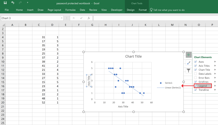
How to Make a Scatter Plot in Excel and Present Your Data Add Labels to Scatter Plot Excel Data Points. You can label the data points in the X and Y chart in Microsoft Excel by following these steps: Click on any blank space of the chart and then select the Chart Elements (looks like a plus icon). Then select the Data Labels and click on the black arrow to open More Options.
Scatter Chart in Excel (Examples) | How To Create Scatter Chart in Excel?
Create an X Y Scatter Chart with Data Labels - YouTube How to create an X Y Scatter Chart with Data Label. There isn't a function to do it explicitly in Excel, but it can be done with a macro. The Microsoft Kno...

How to Make Scatter Charts in Excel - Uses | Features
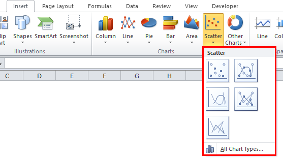
Scatter Chart in Excel (Examples) | How To Create Scatter ... To apply the scatter chart by using the above figure, follow the below-mentioned steps as follows. Step 1 – First, select the X and Y columns as shown below. Step 2 – Go to the Insert menu and select the Scatter Chart. Step 3 – Click on the down arrow so that we will get the list of scatter chart list which is shown below.

Advanced Graphs Using Excel : Shading under a distribution curve (eg. normal curve) in excel
How to use a macro to add labels to data points in an xy ... In Microsoft Office Excel 2007, follow these steps: Click the Insert tab, click Scatter in the Charts group, and then select a type. On the Design tab, click Move Chart in the Location group, click New sheet , and then click OK. Press ALT+F11 to start the Visual Basic Editor. On the Insert menu, click Module.

3d scatter plot for MS Excel
How to display text labels in the X-axis of scatter chart ... Display text labels in X-axis of scatter chart Actually, there is no way that can display text labels in the X-axis of scatter chart in Excel, but we can create a line chart and make it look like a scatter chart. 1. Select the data you use, and click Insert > Insert Line & Area Chart > Line with Markers to select a line chart. See screenshot: 2.
Excel Dot Plots and other charts to display students data
How to Create a Quadrant Chart in Excel - Automate Excel We're almost done. It's time to add the data labels to the chart. Right-click any data marker (any dot) and click "Add Data Labels." Step #10: Replace the default data labels with custom ones. Link the dots on the chart to the corresponding marketing channel names. To do that, right-click on any label and select "Format Data Labels."
Scatter chart · Excelize Document

Scatter Chart in Excel (Uses, Examples) | How To Create Scatter Chart?

Excel Scatter Charts Part 2 - YouTube

How to Add a Third Y-Axis to a Scatter Chart | EngineerExcel
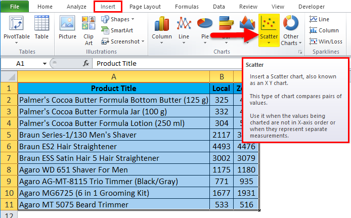
Scatter Chart in Excel (Examples) | How To Create Scatter Chart in Excel?
Post a Comment for "39 scatter chart in excel with labels"